A Roundabout Exposition of Circle Packing

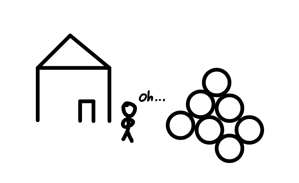
Suppose, rather inconveniently, someone left a handful of unit circles in front of your small abode. Beside the pile was a note, which read: “Please hold on to these circles for an extended period of time.” Begrudgingly, you think about the best way to arrange these circles in such a way that they take up the least amount of space. Do not fret, for this is the problem of circle packing, a well-studied problem under the broader class of packing problems.

Figure 1. An unfortunate situation, with a mathematical solution.

This post aims to give an overview on circle packing along with some interesting results that have been obtained in this field. We assume no specific prior knowledge of the reader other than a basic understanding of geometry.

At its core, packing problems are an optimization problem. They seek to find the best way to arrange a given set of objects in a given space. The primary measure of success is packing density. That is, the ratio of the total area of the packed objects to the area of the space they are packed in. We are interested in finding the optimal packing that grants the highest packing density.

In this post, we will focus on the problem of identifying the optimal packing of circles in a lattice arrangement. We roughly follow the proof outlined in [1], filling in some elementary details and providing some additional intuition along the way.

1. From Circles to Hexagons: The Optimal Packing

1.1. Building Blocks (or Circles?)

First, we begin with a definition of a lattice.

We note that lattices may be defined in higher dimensions, but for the purposes of this post, we are primarily interested in the two-dimensional case. Specifically, two-dimensional lattices over $\mathbb{R}^2$.

We can essentially think of a lattice as a grid of points that extends infinitely in all directions. Importantly, the points in a lattice are arranged in a regular, repeating pattern. The points on the lattice will serve as the centers of the circles that we will be packing. From this, our problem becomes finding the lattice arrangement that allows us to pack the circles with the highest density.

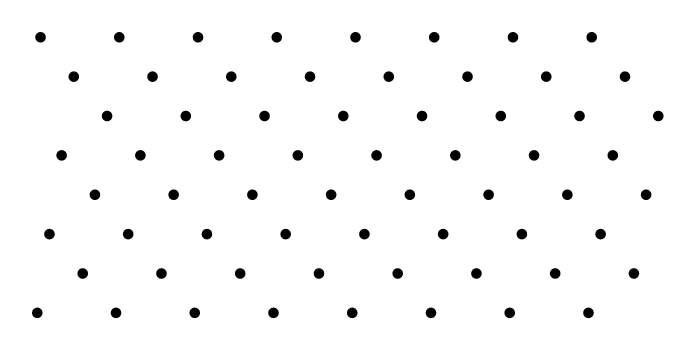
Figure 2. Lattice with $v_1 = (1, 0)$ and $v_2 = \left(\frac{\sqrt{3}}{3}, \frac{1}{2}\right)$.

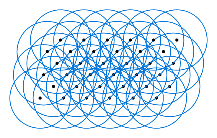
Suppose we were given a lattice $\Lambda$ and we centered a circle with radius $r$ at each point in the lattice. What is the largest radius $r$ such that no two circles overlap?

Figure 3. Lattice with circles centered at each point. The circles overlap, so $r$ is too large.

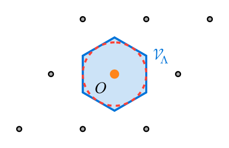
Figure 3 clearly shows that if we choose a radius $r$ that is too large, the circles will overlap. This motivates the idea of a Voronoi cell.

In other words, $\mathcal{V}_\Lambda$ is the set of points that are closer to $O$ than to any other point in the lattice $\Lambda$. We can observe that if we place a circle at $O$, we would want all of its points to be contained within $\mathcal{V}_\Lambda$. Hence, $\mathcal{V}_\Lambda$ gives us an upper bound on the area within which we place our circle.

Figure 4. The Voronoi cell $\mathcal{V}_\Lambda$ (blue, shaded) around the origin $O$ for a hexagonal lattice. The inscribed circle (red, dashed) has radius $r(\Lambda)$.

It turns out that the circle inscribed within $\mathcal{V}_\Lambda$ is the largest circle that can be placed at $O$ without overlapping with any other circles centered at other points in the lattice, motivating the following lemma.

Proof. Let $\Lambda$ be a lattice and $l \in \Lambda$. Let

$$d = \min_{x \in \Lambda \setminus \{l\}} \lVert x - l \rVert$$

be the distance from $l$ to its nearest other lattice point. Due to the repeating, grid-like structure of the lattice, $d$ is the same for every point in the lattice, so we can just consider $l$ without loss of generality. We note that two circles of radius $r$ centered at $l$ and $l' \in \Lambda$ do not overlap if and only if $\lVert l - l' \rVert \geq 2r$. Thus, we have an upper bound $r \leq \frac{\lVert l - l' \rVert}{2}$ for every $l' \in \Lambda \setminus \{O\}$, which is equivalent to $r \leq \frac{d}{2}$.

We claim that $\frac{d}{2}$ is exactly the in-radius of $\mathcal{V}_\Lambda$. The boundary of $\mathcal{V}_\Lambda$ lies on the perpendicular bisectors of segments from $l$ to other lattice points $l' \in \Lambda$; the bisector for $l'$ is at distance $\frac{\lVert l - l' \rVert}{2}$ from $l$. The closest such bisector is therefore at distance $\frac{d}{2}$, which is the in-radius of $\mathcal{V}_\Lambda$. Hence, the largest non-overlap radius equals the in-radius of $\mathcal{V}_\Lambda$.

Working within Voronoi cells allows us to express the overall packing density of a lattice in terms of the area of the Voronoi cell and the area of the inscribed circle. That is,

$$\Delta(\Lambda) = \frac{\text{area of one circle}}{\text{area of Voronoi cell}}.$$

Calculating the area of a circle is straightforward, but how do we calculate the area of a Voronoi cell? To do so, we employ the concept of fundamental domains.

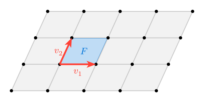
Figure 5. The parallelogram fundamental domain $F$ (blue) formed by basis vectors $v_1, v_2$.

Proof. We first prove that $\mathcal{V}_\Lambda$ is $\Lambda$-covering. Let $P \in \mathbb{R}^2$ be an arbitrary point. We know that there exists a point $l \in \Lambda$ that is closest to $P$. Consider $f = P - l$. We claim that $f \in \mathcal{V}_\Lambda$. Since $l$ is the closest point in $\Lambda$ to $P$, we have $\lVert P - l \rVert \leq \lVert P - x \rVert$ for every $x \in \Lambda$. Then, $\lVert f - O \rVert = \lVert P - l \rVert \leq \lVert P - x \rVert = \lVert f - (x - l) \rVert$ for every $x \in \Lambda$. Since $x$ is an arbitrary point in $\Lambda$, $x - l$ is also an arbitrary point in $\Lambda$ (since $\Lambda$ is closed under addition and negation). Thus, we know $\lVert f - O \rVert \leq \lVert f - x' \rVert$ for every $x' \in \Lambda$, which means $f \in \mathcal{V}_\Lambda$. Since we started with $f = P - l$, we can rewrite this as $P = l + f$ where $l \in \Lambda$ and $f \in \mathcal{V}_\Lambda$, proving that $\mathcal{V}_\Lambda$ is $\Lambda$-covering.

Next, we prove that $\mathcal{V}_\Lambda$ is $\Lambda$-packing. Note that for $l \in \Lambda$ we have

$$l + \mathcal{V}_\Lambda = \{ l + f : f \in \mathcal{V}_\Lambda \}.$$

Let $l_1, l_2 \in \Lambda$ with $l_1 \neq l_2$, and suppose $x \in (l_1 + \mathcal{V}_\Lambda) \cap (l_2 + \mathcal{V}_\Lambda)$. Then $x - l_1 \in \mathcal{V}_\Lambda$ and $x - l_2 \in \mathcal{V}_\Lambda$. Applying the defining inequality of $\mathcal{V}_\Lambda$ to $x - l_1$ with the lattice point $l_2 - l_1 \in \Lambda$:

$$\lVert x - l_1 \rVert = \lVert (x - l_1) - O \rVert \leq \lVert (x - l_1) - (l_2 - l_1) \rVert = \lVert x - l_2 \rVert.$$

Symmetrically, applying it to $x - l_2$ with the lattice point $l_1 - l_2 \in \Lambda$:

$$\lVert x - l_2 \rVert \leq \lVert x - l_1 \rVert.$$

Combining, $\lVert x - l_1 \rVert = \lVert x - l_2 \rVert$, meaning $x$ lies on the perpendicular bisector of the segment $\overline{l_1 l_2}$ which is a line in $\mathbb{R}^2$, hence a set of 2-dimensional Lebesgue measure zero. Therefore $(l_1 + \mathcal{V}_\Lambda) \cap (l_2 + \mathcal{V}_\Lambda)$ has measure zero.

Henceforth, we have shown that $\mathcal{V}_\Lambda$ is both $\Lambda$-covering and $\Lambda$-packing, so $\mathcal{V}_\Lambda$ is a fundamental domain for $\Lambda$.

It turns out that all fundamental domains of a lattice have the same area [2]. Since both a Voronoi cell and $F_\text{par}$ from Example 1 are fundamental domains for $\Lambda$, they must have the same area. Thus, we can prove Lemma 3 which gives us a way to calculate the area of a Voronoi cell.

Proof. From Theorem 8 in [2], we know that all fundamental domains of a lattice have the same area. Since both $\mathcal{V}_\Lambda$ and $F_\text{par}$ are fundamental domains for $\Lambda$, they have the same area.

Hence, we can express the packing density of a lattice $\Lambda$ as

$$\Delta(\Lambda) = \frac{\pi r(\Lambda)^2}{\lvert \det(\Lambda) \rvert}$$

where $r(\Lambda)$ is the radius of the inscribed circle of $\mathcal{V}_\Lambda$. Our goal then becomes identifying the lattice $\Lambda$ that maximizes $\Delta(\Lambda)$.

Our overall proof strategy to optimizing $\Delta(\Lambda)$ is as follows:

1. Reduce all lattices to WR lattices (explained in the next section). For any lattice $\Lambda$, we can construct $\Lambda_\text{WR}$ such that $\Delta(\Lambda_\text{WR}) \geq \Delta(\Lambda)$.
2. Optimize over the space of WR lattices. We show that the formula for $\Delta(\Lambda)$ simplifies significantly for WR lattices, allowing for easy optimization. The subsequent solution is thus the optimal lattice packing of circles.

1.2. Rounding out the Lattices

The core of our proof relies on the concept of Well-Rounded (WR) Lattices. These are a special kind of lattice that satisfy a certain “roundness” condition. In prose, a WR lattice is a lattice such that if we were to draw a circle centered at the origin and gradually increase its radius until it hits any lattice point, the circle would not stop at just one lattice point, but it would stop at two (linearly independent) lattice points at the same time. We shall formalize this intuition with the following definition.

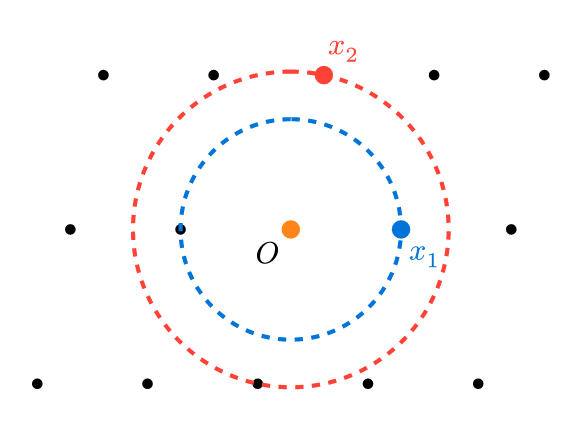
In other words, $\lambda_i(\Lambda)$ is the smallest radius such that the circle of that radius centered at the origin contains $i$ non-zero, linearly independent lattice point(s).

Figure 6. Circles with radius of successive minima $\lambda_1$ (blue) and $\lambda_2$ (red). The circle of radius $\lambda_1$ first touches a lattice point $x_1$; the circle of radius $\lambda_2$ first contains a second linearly independent point $x_2$.

It should be clear that for any $\Lambda$, we must have $\lambda_1(\Lambda) \leq \lambda_2(\Lambda)$. Furthermore, throughout this post, given $x_1, x_2$ corresponding to successive minima, we replace $x_2$ with $-x_2$ if necessary to ensure that the angle between $x_1$ and $x_2$ is $\theta \in [0, \frac{\pi}{2}]$.

We are specifically interested in the case where $\lambda_1(\Lambda) = \lambda_2(\Lambda)$; the lattices that satisfy this condition are called WR lattices.

We can also use the notion of successive minima defined in Definition 4 to express the packing density $\Delta(\Lambda)$ in terms of $\lambda_1(\Lambda)$. That is, the radius of the inscribed circle of $\mathcal{V}_\Lambda$ is given by $\frac{\lambda_1(\Lambda)}{2}$. Hence, $r(\Lambda) = \frac{\lambda_1(\Lambda)}{2}$ and it follows,

$$\Delta(\Lambda) = \frac{\pi r(\Lambda)^2}{\lvert \det(\Lambda) \rvert} = \frac{\pi \lambda_1(\Lambda)^2}{4 \lvert \det(\Lambda) \rvert}.$$

Of course, not all lattices are WR lattices. So, the next thing we want to do is find a way to “round out” any lattice $\Lambda$ into a WR lattice. To do so, we must make the observation that the corresponding successive minima vectors $x_1, x_2$ of some lattice $\Lambda$ form a basis for $\Lambda$. This result was proven in [1, Lemma 3.3] which we restate as Lemma 4.

Also proved in [1] is the following result.

Lemma 5 gives us a concrete way to transform any lattice $\Lambda$ into a WR lattice $\Lambda_\text{WR}$. Importantly for our purposes, $\Lambda_\text{WR}$ has the same first successive minimum as $\Lambda$. This leads us to our next lemma.

Proof. Let $\Lambda$ be a lattice with successive minima $\lambda_1(\Lambda)$ and $\lambda_2(\Lambda)$ and corresponding basis vectors $x_1, x_2$, respectively. By Lemma 4, we know that $x_1, x_2$ form a basis for $\Lambda$. Then, we apply the transformation given in Lemma 5 with $x_1$ and $x_2$ as basis to obtain a WR lattice $\Lambda_\text{WR}$ such that $\lambda_1(\Lambda_\text{WR}) = \lambda_1(\Lambda)$. Let $y_1, y_2$ be the corresponding successive minima vectors for $\Lambda_\text{WR}$ (and also basis by Lemma 4 of $\Lambda_\text{WR}$).

We note that the transformation preserves the directions of the basis vectors; $y_1$ is just $x_1$ and $y_2$ is just a scaled version of $x_2$ and $\frac{\lambda_1(\Lambda)}{\lambda_2(\Lambda)}$ is positive. Hence, the angle $\theta$ between $x_1$ and $x_2$ is the same as the angle between $y_1$ and $y_2$.

It follows,

$$\begin{aligned} \Delta(\Lambda) &= \frac{\pi \lambda_1(\Lambda)^2}{4 \lvert \det(\Lambda) \rvert} \\ &= \frac{\pi \lVert x_1 \rVert^2}{4 \lvert \det(\Lambda) \rvert} && \text{[By Definition 4]} \\ &= \frac{\pi \lVert x_1 \rVert^2}{4 \lVert x_1 \rVert \lVert x_2 \rVert \sin\theta} \\ &= \frac{\lVert x_1 \rVert}{\lVert x_2 \rVert} \cdot \frac{\pi}{4 \sin\theta}. \end{aligned}$$

It also follows,

$$\begin{aligned} \Delta(\Lambda_\text{WR}) &= \frac{\pi \lambda_1(\Lambda_\text{WR})^2}{4 \lvert \det(\Lambda_\text{WR}) \rvert} \\ &= \frac{\pi \lVert y_1 \rVert^2}{4 \lvert \det(\Lambda_\text{WR}) \rvert} && \text{[By Definition 4]} \\ &= \frac{\pi \lVert y_1 \rVert^2}{4 \lVert y_1 \rVert \lVert y_2 \rVert \sin\theta} && [\theta \text{ is the angle between } y_1, y_2] \\ &= \frac{\pi \lVert y_1 \rVert^2}{4 \lVert y_1 \rVert^2 \sin\theta} && [\Lambda_\text{WR} \text{ is WR, so } \lVert y_1 \rVert = \lVert y_2 \rVert] \\ &= \frac{\pi}{4 \sin\theta}. \end{aligned}$$

Finally, since by Definition 4 we have $\lambda_1(\Lambda) \leq \lambda_2(\Lambda)$ and thus $\lVert x_1 \rVert \leq \lVert x_2 \rVert$ which means $\frac{\lVert x_1 \rVert}{\lVert x_2 \rVert} \leq 1$, it follows that

$$\Delta(\Lambda_\text{WR}) = \frac{\pi}{4 \sin\theta} \geq \frac{\lVert x_1 \rVert}{\lVert x_2 \rVert} \cdot \frac{\pi}{4 \sin\theta} = \Delta(\Lambda).$$

Therefore, we have shown that for any lattice $\Lambda$, there exists a WR lattice $\Lambda_\text{WR}$ such that $\Delta(\Lambda_\text{WR}) \geq \Delta(\Lambda)$.

Proof. Suppose for the sake of contradiction that the optimal packing density is achieved by a lattice $\Lambda$ that is not a WR lattice. By Lemma 6, there exists a WR lattice $\Lambda_\text{WR}$ such that $\Delta(\Lambda_\text{WR}) \geq \Delta(\Lambda)$. Since $\Lambda$ achieves the optimal packing density, then we must have $\Delta(\Lambda_\text{WR}) = \Delta(\Lambda)$. Thus, as shown in the proof of Lemma 6, we have

$$\Delta(\Lambda_\text{WR}) = \Delta(\Lambda) \implies \frac{\pi}{4 \sin\theta} = \frac{\lVert x_1 \rVert}{\lVert x_2 \rVert} \cdot \frac{\pi}{4 \sin\theta} \implies \lVert x_1 \rVert = \lVert x_2 \rVert$$

where $x_1, x_2$ are the corresponding successive minima vectors for $\Lambda$ and $\theta$ is the angle between $x_1$ and $x_2$. So, $\lVert x_1 \rVert = \lVert x_2 \rVert \implies \lambda_1(\Lambda) = \lambda_2(\Lambda)$, which means $\Lambda$ is a WR lattice, contradicting our initial assumption.

Therefore, we can restrict our search for the optimal packing density to only WR lattices. This benefits us greatly as the formula for $\Delta(\Lambda_\text{WR})$ where $\Lambda_\text{WR}$ is a WR lattice simplifies to $\Delta(\Lambda_\text{WR}) = \frac{\pi}{4 \sin\theta}$ as shown in the proof of Lemma 6. Thus, our task becomes finding the angle $\theta$ between the two basis vectors of a WR lattice that minimizes $\sin\theta$, which is equivalent to maximizing $\Delta(\Lambda_\text{WR})$.

1.3. Optimizing over Well-Rounded Lattices

With $\theta \in [0, \frac{\pi}{2}]$, the $\sin\theta$ term in $\Delta(\Lambda_\text{WR}) = \frac{\pi}{4 \sin\theta}$ is minimized when $\theta$ is minimized. Thus, we must first place a lower bound on the angle $\theta$ between the two basis vectors of a lattice, motivating the following lemma.

Proof. Suppose towards contradiction that $\theta < \frac{\pi}{3}$. Using a standard linear algebra result, we know $\cos\theta = \frac{x_1 \cdot x_2}{\lVert x_1 \rVert \lVert x_2 \rVert}$. Since $0 \leq \theta < \frac{\pi}{3}$, we have $\cos\theta > \frac{1}{2}$. It follows that

$$\frac{x_1 \cdot x_2}{\lVert x_1 \rVert \lVert x_2 \rVert} > \frac{1}{2} \implies 2(x_1 \cdot x_2) > \lVert x_1 \rVert \lVert x_2 \rVert.$$

Continuing, we expand the following

$$\begin{aligned} \lVert x_1 - x_2 \rVert^2 &= (x_1 - x_2) \cdot (x_1 - x_2) = \lVert x_1 \rVert^2 + \lVert x_2 \rVert^2 - 2(x_1 \cdot x_2) \\ &< \lVert x_1 \rVert^2 + \lVert x_2 \rVert^2 - \lVert x_1 \rVert \lVert x_2 \rVert = (\lVert x_1 \rVert^2 - \lVert x_1 \rVert \lVert x_2 \rVert) + \lVert x_2 \rVert^2. \end{aligned}$$

By Definition 4, we have $\lambda_1(\Lambda) \leq \lambda_2(\Lambda)$ and thus $\lVert x_1 \rVert \leq \lVert x_2 \rVert$. Then, $\lVert x_1 \rVert^2 = \lVert x_1 \rVert \lVert x_1 \rVert \leq \lVert x_1 \rVert \lVert x_2 \rVert \implies \lVert x_1 \rVert^2 - \lVert x_1 \rVert \lVert x_2 \rVert \leq 0$. Thus, it follows

$$\lVert x_1 - x_2 \rVert^2 < \lVert x_2 \rVert^2 \implies \lVert x_1 - x_2 \rVert < \lVert x_2 \rVert.$$

However, we note that this is a contradiction. Since $x_1$ and $x_2$ are distinct and linearly independent, $x_1 - x_2$ is a non-zero vector in $\Lambda$. We also know that $x_1 - x_2$ is linearly independent from $x_1$ since $x_1$ and $x_2$ are linearly independent. $\lVert x_1 - x_2 \rVert < \lVert x_2 \rVert$ tells us then that $x_1 - x_2$ is a non-zero vector in $\Lambda$ that is linearly independent from $x_1$ and is shorter than $x_2$, contradicting the fact that $x_2$ realizes the second successive minimum $\lambda_2(\Lambda)$, i.e. that $x_2$ is the shortest non-zero vector in $\Lambda$ linearly independent from $x_1$. Therefore, we must have $\theta \geq \frac{\pi}{3}$.

We also need a partial converse of Lemma 7: if a basis has equal-length vectors with an angle in $[\frac{\pi}{3}, \frac{\pi}{2}]$, then it already realizes the successive minima. This was proven as Lemma 3.5 in [1], which we restate as Lemma 8.

Next, we can give an example of a WR lattice that achieves the lower bound of $\theta$, motivating the following theorem.

Proof. By Corollary 1, the optimal packing density is achieved by some WR lattice, and the proof of Lemma 6 shows that for any WR lattice $\Lambda_\text{WR}$, $\Delta(\Lambda_\text{WR}) = \frac{\pi}{4 \sin\theta}$, where $\theta \in [0, \frac{\pi}{2}]$ is the angle between the two basis vectors. By Lemma 7, $\theta \geq \frac{\pi}{3}$, so $\sin\theta \geq \frac{\sqrt{3}}{2}$, with equality (hence $\Delta$ maximized) precisely when $\theta = \frac{\pi}{3}$. We claim $\Lambda_\text{hex}$ realizes this optimum. Let $x_1 = (1, 0)$ and $x_2 = \left(\frac{1}{2}, \frac{\sqrt{3}}{2}\right)$.

_$\Lambda_\text{hex}$ is a WR lattice with basis angle $\frac{\pi}{3}$._ Compute $\lVert x_1 \rVert^2 = 1$ and $\lVert x_2 \rVert^2 = \frac{1}{4} + \frac{3}{4} = 1$, so $\lVert x_1 \rVert = \lVert x_2 \rVert = 1$. The angle between them satisfies

$$\cos\theta = \frac{x_1 \cdot x_2}{\lVert x_1 \rVert \lVert x_2 \rVert} = \frac{1 \cdot \frac{1}{2} + 0 \cdot \frac{\sqrt{3}}{2}}{1 \cdot 1} = \frac{1}{2},$$

so $\theta = \frac{\pi}{3} \in [\frac{\pi}{3}, \frac{\pi}{2}]$. By Lemma 8, $x_1, x_2$ correspond to the successive minima of $\Lambda_\text{hex}$, and $\Lambda_\text{hex}$ is WR. Therefore

$$\Delta(\Lambda_\text{hex}) = \frac{\pi}{4 \sin\frac{\pi}{3}} = \frac{\pi}{2\sqrt{3}} \approx 0.9069,$$

and this is the optimal packing density of circles in a lattice arrangement in $\mathbb{R}^2$.

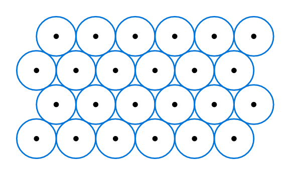
Therefore, we have shown that the optimal packing density of circles in a lattice arrangement is achieved by the hexagonal lattice, with packing density approximately $0.9069$.

Figure 7. $\Lambda_\text{hex}$ with circles centered at each point.

2. Concluding Remarks

In this post, we proved the optimal packing density of circles under the restriction of a lattice arrangement. Rather remarkably, it turns out that if we lift the lattice restriction, the optimal packing density of circles in $\mathbb{R}^2$ is still achieved by the hexagonal packing arrangement. While outside of the scope of this post, the proof of this more general result was first published by Axel Thue; however, his proof was considered incomplete and was not widely accepted until László Fejes Tóth published a complete proof in 1942 [4].

The circle packing problem has also been extensively studied across higher dimensions (sphere packing). More recently, the sphere packing problem in $8$ and $24$ dimensions was solved by Maryna Viazovska and collaborators, with the optimal packings in these dimensions being the $E_8$ lattice and the Leech lattice, respectively [5, 6].

While, clearly, this post represents only a sliver of the rich literature on packing problems, it illuminates some of the key techniques, terminology, and vocabulary that are commonly used in the field. Furthermore, while particularly useful for packing problems, lattices, Voronoi cells, and fundamental domains are also widely used in other areas of mathematics, such as number theory and cryptography. They find use-cases in more applied fields as well, such as coding theory and communications. Overall, the study of packing problems and the associated mathematical tools is a vibrant area of research with deep connections to many other fields.

References

[1] L. Fukshansky. Revisiting the hexagonal lattice: on optimal lattice circle packing. arXiv:0911.4106, 2009.

[2] D. Dadush and L. Ducas. Mastermath, Intro to Lattice Algorithms & Cryptography, CWI Amsterdam, 2018.

[3] T. Tao. An Introduction to Measure Theory. American Mathematical Society, 2011.

[4] H.-C. Chang and L.-C. Wang. A Simple Proof of Thue’s Theorem on Circle Packing. arXiv:1009.4322, 2010.

[5] M. Viazovska. The sphere packing problem in dimension 8. arXiv:1603.04246, 2017.

[6] H. Cohn, A. Kumar, S. D. Miller, D. Radchenko, and M. Viazovska. The sphere packing problem in dimension 24. arXiv:1603.06518, 2017.

Footnotes

1. Lebesgue measure zero is a technical condition that essentially means that the intersection of $l_1 + F$ and $l_2 + F$ is negligible in terms of area [3]. ↩